As a response to a comment on a previous blog post on how to extract SSAS Multidimensional [MD] databases with PowerShell, I decided to write a new blog post, to address the tabular version [Tab].
The main differences working with MD and Tab, programatically, is that MD is represented by XML for Analysis and Tab is using JSON. In management studio this makes no difference however, as you paste XMLA and JSON using the same query type; XMLA (I wonder when/if that will change?)
Obviously, the two technologies MD and Tab are vastly different in almost every other aspect as well, but for the scope of this exercise, we will keep it at that.
Just as in the previous example, we will be using the ability to load assemblies in PowerShell and leverage the functionality the product team has provided. With Analysis Services comes a library of objects to programatically access and manage an Analysis Services instance.
In this documentation, you can dig into the details of options available. All of this extensible from both C# and PowerShell.
Now, back to the problem at hand. We wanted to extract the models from one or more servers, to deploy to another (single) server them or even just persist them locally. To do this, we need to load the Tab version of the assembly, which is that first difference to the original script. Next we need to leverage different functionality within the assembly, to export the json.
The script in all it’s simplicity 🙂
#Load the Tabular version of the assembly
[System.Reflection.Assembly]::LoadWithPartialName("Microsoft.AnalysisServices.Tabular") >$NULL

#Add a comma seperated list of servers here
$SourceServers = @( "<SOURCE SERVERS HERE>" ); #Source
#Add a single server here
$TargetServer = "<TARGET SERVER HERE>"; #Target

cls;

#Uncomment to deploy to target server
#$TargetServer.Connect();

#Loop servers
ForEach( $srv in $SourceServers ) {

    #Connect to current server
    $server = New-Object Microsoft.AnalysisServices.Server
    $server.connect($srv)

    #Loop al databases on current server
    ForEach(  $database in $server.Databases ) {

        #Generate Create Script - Other options are available, see https://docs.microsoft.com/en-us/dotnet/api/microsoft.analysisservices.tabular.jsonscripter?view=analysisservices-dotnet
        $json = [Microsoft.AnalysisServices.Tabular.JsonScripter]::ScriptCreate($database, $false)

        #Create Path
        $Path = "<INSERT DUMP LOCATION AND FILE NAME>" + ".json";

        #Export the model to file
        $json | out-file -filepath $Path

        #Uncomment to deploy to target server
        #$TargetServer.Execute($json);
    }
}
There are a lot of great examples out there on how to build your own custom Time Intelligence into Analysis Services (MD). Just have a look at this, this, this, this and this. All good sources for solid Time Intelligence in SSAS.
One thing they have in common though, is that they all make the assumption that there is and will always be 52 weeks in a year. The data set I am currently working with is built on ISO 8601 standard. In short, this means that there is an (re-) occurrence of a 53rd full week as opposed to only 52 in the Gregorian version which is defined by: 1 Gregorian calendar year = 52 weeks + 1 day (2 days in a leap year).
The 53rd occurs approximately every five to six years, though this is not always the case. The last couple of times we saw 53 weeks in a year was in 1995, 2000, 2006, 2012 and 2015. Next time will be in 2020. This gives you enough time to either forget about the hacks and hard-coded fixes in place to mitigate the issue OR bring your code in a good state, ready for the next time. I urge you do the latter as suggested by the work philosophy of the late Mærsk McKinney Møller: Constant Care.
The Real Issue
So why is this such a big deal? After all, it’s only a problem every say five-six years.
For starters, some built-in functions in Analysis Services will go bunkers over this sudden alienated week.
Your otherwise solid calculations will suddenly have wholes, blanks and nulls in them. The perfect line chart broken. Not to mention the Pie chart, where a perhaps crucial piece is missing!
In my line of work there have been a great deal of discussion about how to treat this troublesome Week 53. One suggestion was to just distribute the sale on Week 53 to all other weeks across the year. Every week thereby containing a fraction (1/52) more sale than usually – this way, comparison across years will even out. But what about companies that have a huge spike in sales around New Years Eve (think Liquor) – they would then not be able to compare the real sale around New Years Eve, because this would be disguised by the massive sale over the rest of the year.
Our working solution is to compare the same number of weeks as the current year you are operating with. In 2016 that’s 52 weeks, in 2015 it was 53 weeks.
The tricky part about this is to identify when to calculate what, and for this we need assistance from additional attributes in our calendar dimension.
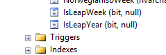
New attributes to support this type of calculation are [Is Leap Week] and [Is Leap Year].
Is Leap Week has the value 1 whenever the current week is the 53rd week of the year. All other weeks are represented by a 0.
Is Leap Year has a value of 1 whenever the current year consists of 53 weeks. All other years are represented by the value 0. Arguably the name Leap Year could be considered confusing, as this normally means something else. Alternative names could be: Has53Weeks, HasExtraWeek or something along those lines.
Getting Set Up
You database table should look something along the lines of this:
Another table is needed for the Time Intelligence to work it’s magic – This one is for the members of the something along the lines of the Date Tool Dimension by Alberto Ferrari (b|l|t) and Marco Russo (b|l|t) which can be found here. My implementation differs a little bit, here’s how.
I have one dimension in the cube, named Date Tool. This dimension has two attributes with members accordingly. For one part I’d like to control the calculation in terms of overall scope/length of the calculation, i.e. 4 weeks aggregated or is it 8 weeks? This attribute I have named Aggregation Tool. The other element is when I want the calculation to occur, i.e. Today, Yesterday or Last Year. This attribute I have named Comparison Tool.
Members of the Aggregation Tool are: YTD, YTD LY, Last 4 Weeks, Last 8 Weeks, …, Last 52 Weeks. Members of the Comparison Tool are: Current Period (N), Last Period (N-1), Previous Period (N-2) and some the we actually don’t use.
The fact that the two attributes can be combined behind the scenes in the cube, makes this a very powerful ally.
In the Cube
In the cube we need to address the time intelligence by adding a bit of MDX script. This relies on SCOPE assignments which Chris Webb (b|l|t) has been kind enough to blog about here, present about at SqlBits VIII here, and Pragmatic Works has a video on here.
Now, reminded that we need to address the Week 53 issue and calculate a similar number of weeks to compare with for, in particular, Last Year calculations that stretch across Week 53. Let’s say 2016 Week 1 through 20, what’s the equivalent sale last year? In our case, its 2015 Week 2 through 21.
With a SCOPE statement, it’s possible to bend and twist the calculations as you see fit, and in this case, to right shift the calculation, so to speak. Here is how the calculation should look like.
[Date Tool].[Aggregation Tool].&[1] and [Date Tool].[Comparison Tool].&[1] are the default values, Current Week and Current Period respectively.
The above SCOPE statement is invoked every time the [Date Tool].[Aggregation Tool].&[18] ~ [Date Tool].[Aggregation Tool].[Year To Date Last Year] member is present in a an MDX query. So if this is active in any slicer, this piece of code will be run and the aggregation will be calculated accordingly.
Wrap Up
Before entering the domain of Retail, I would have never thought that periods could vary over time. Except maybe for my time in Government Healthcare where a 13th month was introduced, to right all the wrongs of the year. So, in other words, I guess there are many examples out there, where the good old faithful calendar simply does not cut it. In those cases, the SCOPE assignment in SSAS really does some magic for you. But beware, SCOPE assignments done wrong can get you into serious trouble, leading to all kinds of odd- or subtle miss-calculations that you don’t detect right off the back.
A final word on this approach is, that you should test every corner of your cube, before you trust any of your calculations, when dealing with SCOPE assignments. More times than I cared to count I have been fooled by a SCOPE assignment.
This months T-SQL Tuesday is hosted by Kenneth Fisher(b|l|t) and the invitation is found following this link.
T-SQL Tuesday was started by Adam Machanic (b|t), and this is the SQL Server community’s monthly blog party, where everyone is invited to write about a single common topic. This time, the topic is Backup (and Recovery).
Admitted, I was a bit challenged this past week as I decided to update my WordPress to a newest version 4.7. This however caused the admin module of my site to become unavailable. After creating a support ticket with Unoeuro.com I was guided to a blog post by Vashistha Pathak (b|t) which in the end led me to the solution, and I fixed it without the need of a backup. Phew… Kind of nerve wrecking not knowing if my site was backed up – fortunately I wouldn’t have lost a single character, according to Unoeuro support. That was quite reassuring and somehow coincidentally very fitting for this months topic, no?
My approach for this blog post is to accept Kenneth’s challenge from this tweet, where Kenneth triggered a thought stream using the word keys:
@vestergaardj *nod* I’m hoping to get a really broad spectrum. Everything from basic DB backup, to keys, to BI.
I immediately came to think of SSRS encryption key backup and I knew by then I had to try to cover all basics on BI solutions, this being SSAS, SSIS and SSRS as well. But honestly, I haven’t been able to set aside enough time to cover all. So without further ado, here is SSAS Backup Galore (the others will come in good time):
SSAS (MD)
For Analysis Services databases there are two (2) fairly straight forward options. However, you may want to discuss up front, how much effort you want to spend setting this up. Consider you already have a process for deploying updated cubes into production; In which scenarios would it be alright for the business to wait for a normal deploy, for the numbers to come back online?
In Brent Ozar’s (b|l|t) First Responder Kit there is a document where IT and Business need to state how quickly they would like to recover from different categories of “down time” i.e. Corruption, “Oops” Queries and so on. That’s actually still a good exercise to do, with both sides of the table, even though the document operates at a higher level.
Prerequisites
You must have administrative permissions on the Analysis Services instance or Full Control (Administrator) permissions on the database you are backing up.
Restore location must be an Analysis Services instance that is the same version, or a newer version, as the instance from which the backup was taken.
Restore location must be the same server type.
SSAS does not provide options for differential or partial backups of any kind. Nor log backups (should you be wondering in from the DBA world).
A SSAS backup contains only one (1) database, so no option to create backup sets.
SSAS can only have one fixed backup location at a time; It’s configurable, but not meant to be changed for each database.
GUI
We begin by connecting to the server where the database resides. Via SQL Server management Studio (SSMS) you then expand the Node Databases. In my example here, I will be using a Database named ‘Test Database’.
When right-clicking on the selected database, we get the option to Back Up.
This kicks off a wizard where we need to select a few options for our backup.
First of all, we can edit or designate the name of the backup file. One thing to note with regards to backups on SSAS is that only one designated backup folder can be active at a time. In the server options dialog, it’s possible to change the destination for backups, but only after adding the new folder location to the attribute AllowedBrowsingFolders, which is considered an advanced setting, so remember to tick that option in order to set the new location. Also, you need to do this by opening the dialog twice; 1st add the new folder to AllowedBrowsingFolders, close and reopen. 2nd change the BackupDir to the newly added folder.
My settings are just the standard ones, yours should differ in the sense that you should put your Data, Backup and Log on different disks for optimal performance.
Well, this is why you only get to type a name for the file in the next dialog and not the complete path and file name. You also get to select, if the backup can overwrite an existing file of same name. Tick if you would allow this.
The two other options I will cover in this post are Apply Compression and Encrypt backup file.
I have not met a setup where applying compression was not an option, yet. Obviously this has a penalty cost on CPU while executing the backup, and will affect the rest of the tasks running on the server (even if you have your data and backup dir on different drives). But in my experience, the impact is negligible.
This may not be the case with the encryption option, as this has a much larger foot print on the server. You should be using this with some caution in production. Test on smaller subsets of the data if in doubt.
Another thing to keep in mind, as always when dealing with encryption, do remember the password. There is no way of retrieving the data other than with the proper password.
In my example I allow file overwrite and apply compression.
When we clicking the OK button, the backup will execute and you will be able to track the progress in the lower left corner of the dialog. The dialog will close after successful completion. You have the option to stop the backup action from the progress dialog by clicking Stop action now.
After completion the file should be sitting on disk, where you designated it.
XMLA
Same options as mentioned above in the GUI section are available when doing your backups via XMLA.
Connection to the server, start an XMLA query and fire away.
To leave out Password, just leave out the entire tag. Vice versa goes for Compression which you have to specify with False, in order to not have your backup compressed. In the above example, the backup is compressed.
Often I have seen this used within a SQL Agent job, that support SSAS Commands, just as the one above. Look for the SQL Server Analysis Services Command Step Type.
Obviously setting this up in a SQL Agent job is only half the job. After the backup has been done and/or scheduled, you need to ensure that the backup files produced are stored in a secure and available location.
PowerShell
Via the PowerShell cmdlet Backup-ASDatabase you can execute the same backup as described above. In fact this is a perfect example of why you should learn PowerShell, if your not already on that band wagon. Simply put, it doesn’t get easier than this. In my example, I will create a backup of all the databases on a server, in a couple of lines of code – Behold PowerShell AwesomeSauce (PSAS)
Import-Module sqlps -DisableNameChecking
sqlserver: | Out-Null
cd sqlas |Out-Null
cd <server>\<namedinstance>\databases
dir | Backup-ASDatabase
Remember to exchange your own values for <server> and if present <namedinstance>.
This will backup all databases on the given server.
Obviously you can extend this script with all the parameters exposed by the cmdlet. For more details, see this page.
Analysis Services Management Objects
The final method I will be covering is via Analysis Services Management Objects or AMO for short. AMO exposes, as PowerShell, a great deal of methods, where backup is one.
In order to use AMO to back up an SSAS database we need to get an create or load instance of said database through the object model in AMO. This can be done fairly easy.
The AMO classes/functionality comes with the Microsoft.AnalysisServices.dll which is installed with the product. In order to utilize it, we need to load it first or reference it, if you are doing a proper .Net project in SQL Server Data Tools or Visual Studio.
One thing to note before we go to the example is that the Backup method in the Database object has several implementations. Depending on your parameters, you can call different implementations of the same method. According to Technet, these are your options:
You should note that only via the method that takes a BackupInfo class as parameter are you able to specify a password.
Final thoughts
I think I have covered all possible ways of executing an Analysis Services backup – If I somehow missed and option, please let me know!
But as you can see, ways to back up your SSAS database are abundant and very flexible.
You should, as with any backup, on a regular basis restore and test them on a separate environment, to ensure that you can actually recover when needed.
Depending on data update frequency this can however be rather a complex setup.
This is my twelfth (12th) post in a series of entry-level posts, as suggested by Tim Ford (b|l|t) in this challenge.
I have not set any scope for the topics of my, at least, twelve (12) posts in this blog category of mine, but I can assure, it’ll be focused on SQL Server stuff. This time it’s going to be about how to create an Azure Analysis Services [AAS] Instance via the Azure Portal and connect to it from Power BI.
One of the Microsoft’s biggest announcements at this years PASS Summit, was Azure Analysis Services. Period. CNTK second, IMO. So, why should you care?
According to Microsoft, this is why:
Based on the proven analytics engine in SQL Server Analysis Services, Azure AS is an enterprise grade OLAP engine and BI modeling platform, offered as a fully managed platform-as-a-service (PaaS). Azure AS enables developers and BI professionals to create BI Semantic Models that can power highly interactive and rich analytical experiences in BI tools such as Power BI and Excel. Azure AS can consume data from a variety of sources residing in the cloud or on-premises (SQL Server, Azure SQL DB, Azure SQL DW, Oracle, Teradata to name a few) and surface the data in any major BI tool. You can provision an Azure AS instance in seconds, pause it, scale it up or down (planned during preview), based on your business needs. Azure AS enables business intelligence at the speed of thought! For more details, see the Azure blog.
If you’re still thinking “Nah, it’s no biggie”, you should read it again. This is huge.
Getting it airborne
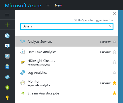
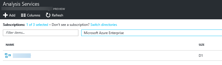
In this example, I will only show how to create the AAS instance from the portal. So we are heading there, right away. The easiest way, is to search in the services search field:
Click the Analysis Services link (as you can see, still in preview) and you will be directed to the, hopefully familiar, service tab/screen in Azure.
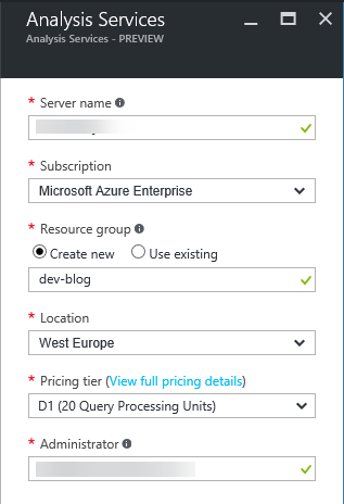
Click Add and you will see the configuration tab to the left
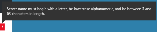
On naming, there are currently? restrictions, so you are down these basic naming rules:
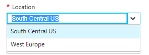
Locations supported are currently only West Europe and South Central US.
Probably the most interesting part (even if you don’t care, someone on a higher pay grade will) is about Pricing Tier. As for now, there are four (4) pricing tiers D1, S1, S2 and S4 (I see what you did there Azure Team; The well-known Windows skip version?) Approximate cost units are 1, 15, 30 and 60 respectfully; So if D1 costs $50 a month, S4 costs $3.000 – as you can see, forgetting to shut down an S4 instance can quickly build up a bill, so beware.
Once you click ‘Create‘ after setting all the configurations, you will be guided back to the service tab and here you’ll see your instance.
Connecting from Power BI
This requires the latest November update from the Power BI Team.
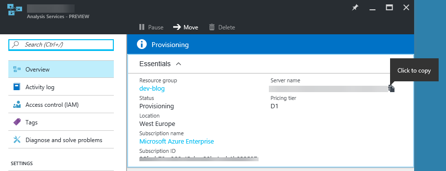
Before you connect, you need to get the server name. In Azure portal > server > Overview > Server name, copy the entire server name.
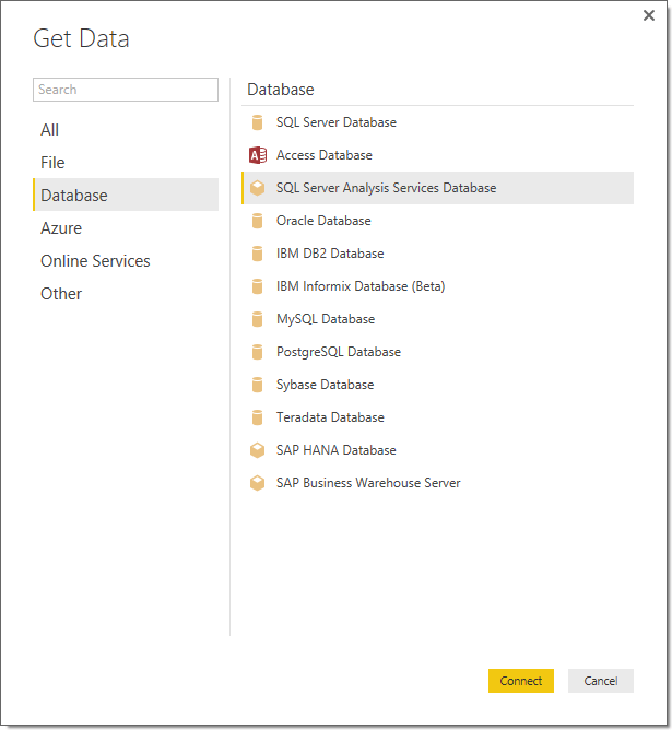
In Power BI Desktop, click Get Data > Databases > Azure Analysis Services.
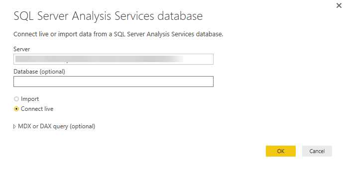
In Server, paste the server name from the clipboard.
In Database, if you know the name of the tabular model database or perspective you want to connect to, paste it here. Otherwise, you can leave this field blank. You can select a database or perspective on the next screen.
Leave the default Connect live option selected, then press Connect. If you’re prompted to enter an account, enter your organizational account.
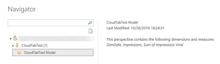
In Navigator, expand the server, then select the model or perspective you want to connect to, then click Connect. A single click on a model or perspective shows all the objects for that view.
During a presentation of mine, there was a discussion going on, about what partitioning strategy to use when partitioning cubes. Most frequently it seems people are partitioning by some form of period, e.g. by Years, Months or Weeks. Rationally it may seem like a good idea, at the time. But wouldn’t it be a more fact based approach to actually put the strategy to a test?
Preface
There are several ways of approaching cube, or more precisely, measure group partitioning. One approach is to simply define the partitions in the Visual Studio Data Tools [SSDT] project and then deploy/process the database for testing. This process is cumbersome and very manual, which in the end, very likely, can lead to erroneous conclusions.
On codeplex, there is a project called ASStoredProcedure which is a collection of Stored Procedures (compiled C# code). By installing the assembly on a given SSAS instance, you get access to use all kinds of cool methods.
For more information on custom assemblies in Analysis Services, read this and this.
The outcome of calling this method is a measure group that is partitioned by the members present in the designated set. In the following example the measure group Internet Sales is going to be partitioned by Year.
It’s important to keep some of the obvious draw backs of this approach in mind.
First of all, you need to have a fully processed cube, in order to execute the method. Having only the measure group and the dimension in question processed is not enough. This means, that if the cube is considerable in size, the pain of processing will be double during the creation of the partitions. Initially process in order to create the partitions, then process the partitions – you can elect to process the cube the second time by Default rather than Full, which will detect changes in the Measure Groups in question and only process those.
Second, if data during a future process, exceeds the given boundaries of the partitions (specified in the slice attribute – which the AS Stored Procedure will set at the time of creation) processing will break. One example could be that the underlying data source provides a rolling window, and if a specified partition has no data, processing will break. This behavior was a bit surprising to me. So you need to re-create partitions on a regular basis. As often as your “grain” on the partitions allow for spill. This is particularly hurtful when/if the whole cube needs re-processing each and every time data is updated.
Semi-Automation
Obviously everyone can execute MDX of the back in SSMS. But the trick is to use PowerShell to do the hard work for you. With a few lines of code, we can easily set up the whole test – you would want to test all your theses.
First we create two helper functions, to assist with the repetitiveness.
Remember to replace <SERVERNAME>, <DATABASENAME> (don’t forget the clear cache XMLA statement),<CUBENAME> and <MEASUREGROUPNAME> with your own values. Also adjust the path for the MDX you want to have run against the cubes. I tried to parametrize the method but for some reason the function failed to convert the input to
When this is in place, we can loop the sets we want our measure group to be partitioned by. In my example, I create the following partition schemes: Year per Datasource, Datasource, Year, Week, Store and finally Chain. This is where your knowledge about both your data demographics and end users query statistics come into play. Remember, partitioning can improve both query and processing.
Depending on the size of your data, this can be quite a time-consuming endeavour, which is why automating it makes a lot of sense.
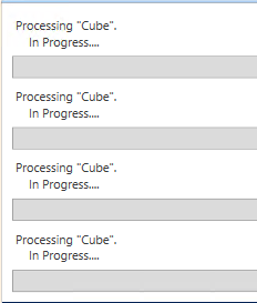
Here’s how the IDE displays the progress
One after another, the cubes are processed. The Write-Host statements are covered by the graphics.
I left out one thing from this example; to test processing durations. This is, however an easy fix, as we can record the time at process begin as well as the time at process end, subtract the two and get the duration. This way, we can check how processing performance is affected by the different partition schemes.
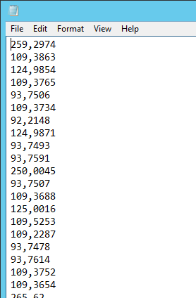
To view the rudimentary outcome, have a look in the file configured in the script. Timings will be listed as a long list of durations, like this:
With this data, you can put your scheme to the test; Find out which partition scheme, if any at all, works best for your particular cube.

 Members of the Comparison Tool are: Current Period (N), Last Period (N-1), Previous Period (N-2) and some the we actually don’t use.

 When right-clicking on the selected database, we get the option to Back Up.